Beating Minesweeper With Neural Networks
This is a project which I completed earlier this year, after a previous attempt trying to beat 2048. The play strategy is relatively simple and can be followed and replicated by beginners in machine learning. All the code is at https://github.com/sn6uv/minesweeper.
This post demonstrates how to acheive good human performance on minesweeper using neural networks to predict mine locations.
Implementing minesweeper
Minesweeper was implemented in Python. Each game state is represented as an
instance of a Game object
class Game:
    def guess(self, pos):
        '''True iff a mine was hit.'''
        ...

    def is_won(self):
        '''True iff the game is won.'''
        ...

    def view(self):
        '''Machine readable representation of what's visible.'''
        ...
see game.py for implementation details. The key ideas are to precompute the neighbors of each position and store the list of mines positions as a set for efficient lookup.
The first move is always safe, so mines are initialised after the first guess.
Learning to play minesweeper
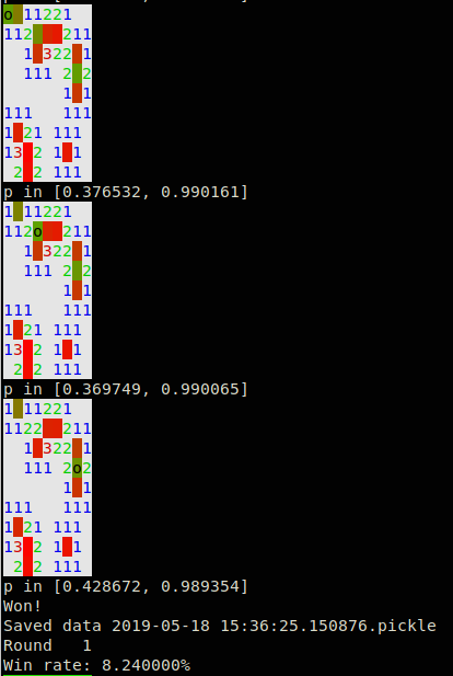
Given an input board the agent predicts the probability of finding a mine at each open location. It selects the lowest probability location for its next guess. This process repeats until until the game is over.
The Agent’s objective is to predict the locations of mines based on a ‘view’ of the game board.
Note that this is not actually an optimal strategy. A higher risk guess may reveal more information about the location of mines, thus leading to a shorter game, and a higher overall win-rate. Winning the game is approximated as not loosing each guess.
This agent (arrow above) is repesented as a Player object
class Player:
    def __init__(self, height, width, mines):
        self.height = height
        self.width = width
        self.mines = mines
        self.data = []
        self.model = Model(height, width)

    def play(self, rounds):
        won = 0
        for _ in range(rounds):
            g = Game(self.height, self.width, self.mines)
            won += self.play_game(g)
        print("Win rate: %f%%" % (100.0 * won / float(rounds)))

    def play_game(self, game):
        hit_mine = False
        while not hit_mine:
            hit_mine = self.play_move(game, debug)
            self.data.append((game.view(), game.mines))
            if game.is_won():
                return True
        return False

    def play_move(self, game):
        view = game.view()
        pred = self.predict_mines(view)
        pos = np.unravel_index(np.argmin(pred), (self.height, self.width))
        if not game.guessed:
            # Randomise first guess to prevent bias, since first mine moves.
            pos = random.randint(
                0, self.height-1), random.randint(0, self.width-1)
        return game.guess(pos)

    def predict_mines(self, view):
        game_input = self.get_model_input(view)
        pred = self.model.predict(game_input)[0]
        pred[view.flatten()!=9]=1    # Ignore alreday guessed locations
        return pred
The first move is always safe in minesweeper so the AI chooses at random to remove bias in the data derived from player initialisation.
The player accumulates data on previous games. This will be used for training
the model. In order to beat minesweeper we will attempt to implement the
predict_mines function using a neural network.
View representation
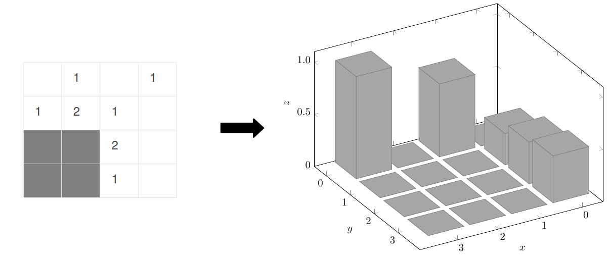
Each tile in the game grid can be either guessed or unguessed. If it’s guessed there is either a bomb or a number of adjacent bombs $0, \dots, 8$. In total, each tile has 10 potential states.
If $h$ is the height of the board and $w$ is the width we define
\begin{equation} n := height \times width \end{equation}
as the input size. Each tile was represented as a one-hot input vector, to give a total input size of $10 n$.
Neural network architecture
The neural network used had 5 fully-connected layers with sizes $[10n, 20n, 10n, 5n, n]$ respectively. Each layer had a ReLU activation except for the final layer which used a sigmoid activation.

This works out to $455n^2 + 46n$ parameters.
The network $f$ takes an input game $x \in \{0,1\}^{10n}$ state and outputs $p \in \mathbb{R}^n$, the probability distribution of mines.
The loss function used was the cross-entropy loss with $L^2$ regularisation,
where $N$ is the total number of samples and $\hat{p}_i \in \{0,1\}^n$ is the true probabilities for training batch $i$.
This architecture was implemented as a Model object using TensorFlow.
class Model:
    def __init__(self, height, width):
        self.height = height
        self.width = width
        self.build_model()
        self.sess = tf.InteractiveSession()
        tf.global_variables_initializer().run()

    def build_model(self, learning_rate=LEARNING_RATE, beta=L2_REGULARISATION):
        n = self.height * self.width
        self.x = tf.placeholder(tf.float32, [None, 10 * n])

        W1 = tf.get_variable('W1', [10 * n, 20 * n])
        b1 = tf.get_variable('b1', [20 * n])
        z1 = tf.matmul(self.x, W1) + b1
        a1 = tf.nn.relu(z1)

        W2 = tf.get_variable('W2', [20 * n, 10 * n])
        b2 = tf.get_variable('b2', [10 * n])
        z2 = tf.matmul(a1, W2) + b2
        a2 = tf.nn.relu(z2)

        W3 = tf.get_variable('W3', [10 * n, 5 * n])
        b3 = tf.get_variable('b3', [5 * n])
        z3 = tf.matmul(a2, W3) + b3
        a3 = tf.nn.relu(z3)

        W4 = tf.get_variable('W4', [5 * n, n])
        b4 = tf.get_variable('b4', [n])
        z4 = tf.matmul(a3, W4) + b4

        self.p = tf.nn.sigmoid(z4)
        self.p_ = tf.placeholder(tf.float32, [None, n])

        loss_p = tf.reduce_mean(tf.reduce_sum(tf.nn.sigmoid_cross_entropy_with_logits(labels=self.p_, logits=z4), reduction_indices=[1]))
        regulariser = tf.nn.l2_loss(W1) + tf.nn.l2_loss(W2) + tf.nn.l2_loss(W3) + tf.nn.l2_loss(W4)

        self.loss = loss_p + beta * regulariser
        self.train_step = tf.train.AdamOptimizer(learning_rate).minimize(self.loss)

    def predict(self, grid):
        """Evaluates the model to predict an output.

        Args:
            grid: a game state as a height*width*10 vector.

        Returns:
            p: probability distribution over moves.
        """
        grid = grid[np.newaxis, :]
        p = self.sess.run([self.p], feed_dict={self.x: grid})
        return p[0]
Training
The model was trained in batches. Metrics are stored in a small utility class:
class ModelBatchResults:
    '''The result of training the model on one batch. '''
    def __init__(self, loss, precision, recall, accuracy):
        ...
Some care has to be taken when paritioning training and test sets, but otherwise training the model is relatively straightforward.
class Model:
    ...
    def train(self, examples, batch_size=5000, epochs=1):
        """Trains the model on examples.

        Args:
            examples: list of examples, each example is of the form (grid, p).
        """

        # Split a fraction of data for testing. Since data comes from playing
        # games, if we take a random subset for testing then it's correlated
        # with the training data. Taking a slice off the end mitigates this.
        num_test_examples = int(len(examples) * 0.01)
        examples, test_examples = examples[:-num_test_examples], examples[-num_test_examples:]
        test_data = list(zip(*test_examples))
        self.measure_batch(*test_data).print_testing()

        for epoch in range(epochs):
            print("Epoch %3i" % epoch)
            random.shuffle(examples)
            results = []
            for idx in range(0, len(examples), batch_size):
                batch = examples[idx:idx+batch_size]
                grids, ps = list(zip(*batch))

                result = self.train_batch(grids, ps)
                results.append(result)

                if idx % PRINT_ITERATIONS < batch_size:
                    ModelBatchResults.combine(results).print_training(idx+batch_size, len(examples))
                    results = []
            if results:
                ModelBatchResults.combine(results).print_training(len(examples), len(examples))
                results = []
            self.measure_batch(*test_data).print_testing()

    def train_batch(self, grids, ps):
        feed_dict = {self.x: grids, self.p_: ps}
        self.sess.run(self.train_step, feed_dict=feed_dict)
        loss = self.sess.run([self.loss], feed_dict=feed_dict)[0]
        pred = self.sess.run([self.p], feed_dict=feed_dict)[0]
        return ModelBatchResults.from_prediction(loss, pred, ps)

    def measure_batch(self, grids, ps):
        feed_dict = {self.x: grids, self.p_: ps}
        loss = self.sess.run([self.loss], feed_dict=feed_dict)[0]
        pred = self.sess.run([self.p], feed_dict=feed_dict)[0]
        return ModelBatchResults.from_prediction(loss, pred, ps)
Metrics are printed at regular intervals to ensure that training is making progress but ultimately sucess is determined by win rate. see model.py for details.
In order to generate training data, the agent plays a series of games and then trains on the resulting game histories.
def play_train(player, play_games, train_epochs, batch_size):
    '''Play a number of games and then train on the resulting data'''
    print("Playing %i games" % play_games)
    player.play(play_games)
    print("Training on %i examples" % len(player.data))
    player.train(batch_size=batch_size, epochs=train_epochs)
    player.data = []
Old game histories are discarded to prevent overfitting. This process repeats iteratively until the desired win-rate is acheived, see learn_from_scratch.py for an example on how to train beginner difficulty to >50% win rate.
The following hyperparamers were used during training:
| symbol | description | value |
| $\alpha$ | Learning rate | 1e-3 |
| $\beta$ | L^2 regularisation coefficient | 1e-4 |
| batch size | 1024 | |
| test set fraction | 1e-2 | |
| training epochs | 1 |
These can be set in config.py.
Results
| height | width | number of mines | win rate | training duration | parameters |
| 4 | 4 | 2 | 90% | <1min | 117216 |
| 5 | 5 | 3 | 80% | 10min | 285525 |
| 9 | 9 | 10 | 80% | 3 days | 2988981 |
The network was trained on core i7-6600U CPU @ 2.60GHz.
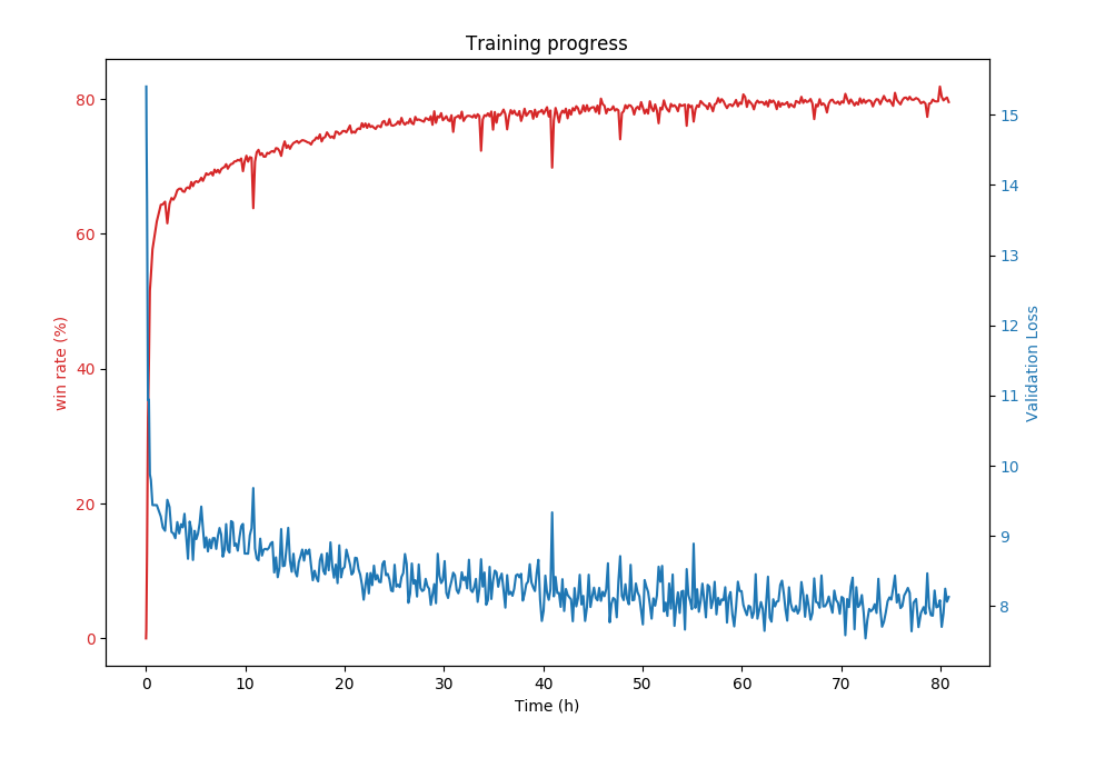
Training progress for beginner board.
This network was tested on larger networks, but the training rate was too slow to get any good results.
Conclusion
This neural network acheives an 80% win rate on the beginner board (9x9 with 10 mines). Anecdotally, this is on par with a good human player.
Training this network is quite slow. Unsuprisingly the bottleneck is the game simulation in Python. Some attempt was made to optimise this but it could be improved significantly by switching to a faster language like C++ or running multiple simulaitons in parallel on a more powerful machine.
Future work
CNNs
By flattening the input board to a $10 \times h \times w$ vector the network needs to learn the spatial relationships between input variables. A convolutional neural network (CNN) might generalise better, especially for larger input boards. Moreover, a CNN trained on one board size could also play on other boards, assuming a simlar mine density. A side-effect would be to reduce the model size.
Reinforcement learning
The goal is to optimise win rate; predicting mine locations is only useful towards that goal. A reinforcemnt learning approach, such as Q-learning might be more effective at increasing the win-rate, at the tradeoff of slower training rate.
Try it yourself
Requires tensorflow and numpy.
git clone https://github.com/sn6uv/minesweeper.git
cd minesweeper
python learn_from_scratch.py